Meteorologists have been leveraging computers to understand and predict the atmosphere for as long as computers have existed. Computer models work by solving a complicated system of equations on a grid spread across the atmosphere. Much like camera pixels, the more grid points you have and the closer you can pack them together, the more details you’ll be able to see.
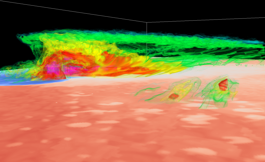
Currently, the highest resolution operational weather model in the United States is the High Resolution Rapid Refresh with a grid spacing of about 3km. Without the constraints of needing to produce a timely forecast for the whole country, I was able to push the grid spacing of WRF down to 333m. At this scale, not only is the storm itself explicitly resolved, but so too are many sub-stormscale processes such as the forward and rear flank downdrafts, the mesocyclone, and sometimes even hints of the wall and tail cloud features that develop underneath the strongest portion of the updraft.
How It’s Done
Computation
These simulations were conducted using the WRF-ARW model running on NCAR’s Cheyenne supercomputer.
The tremendous computing power of Cheyenne allowed me to run the WRF model with nearly 365 million grid points representing a 1102x1102x300 grid over parts of southern Texas where a powerful supercell thunderstorm had dropped 6.5″ hail on the evening of April 28th, 2021.
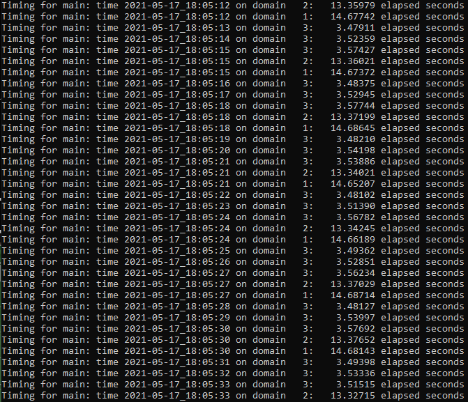
I had to deal with a number of computational challenges running the model at this scale including some serious I/O bottlenecks and numerical instabilities.
Visualization
To visualize the data produced by these simulations, I employed two primary tools: NCAR’s VAPOR software for volumetric renderings and WRF-Python for 2-D images and quantitative insights.
I’ve run VAPOR both on my own computer and on NCAR’s Casper visualization system. While I have been able to produce some renderings using my NVIDIA Quadro-P2000 graphics card, the performance increase offered by Casper’s NVIDIA Quadro-GP100 cards is significant, cutting rendering times more than in half and offering significantly improved interactive performance.

The Value of Higher Resolution
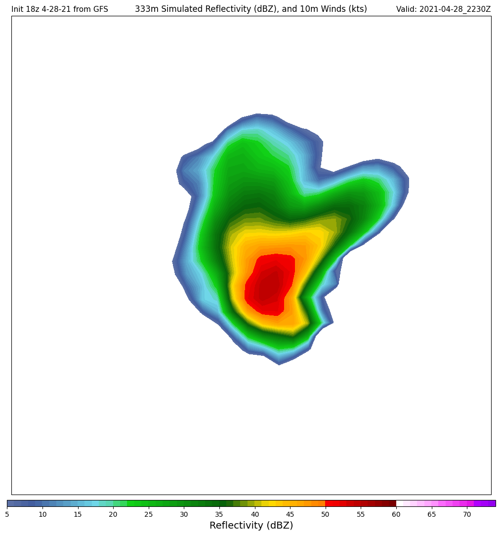
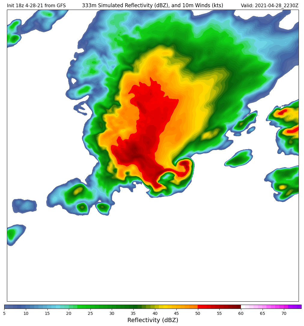
As the slider on the image above demonstrates, there are many details that emerge when the model grid spacing decreases from 3km to 333m. The storm’s hook echo is much better defined, as are fluctuations in the rear flank reflectivity field and smaller cells trailing and leading the main storm.
So why don’t we have 333m models running operationally? The answer is computational cost. For every factor of three you reduce the horizontal resolution (i.e. from 3km to 1km or 1km to 333m), you increase the number of computations the model must make by a factor of 27 (3x in the x-direction, 3x in the y-direction, and 3x in the time dimension because you also need to shrink the time between subsequent computations to prevent numerical instability from taking hold of the model. For some perspective, it took me several days to run this simulation for six hours of “forecast” time (though there is still much I have yet to learn about optimizing performance on machines like Cheyenne).
The analysis of this data is still very much a work in progress, and this page will be updated as I generate new figures.
-Jack
